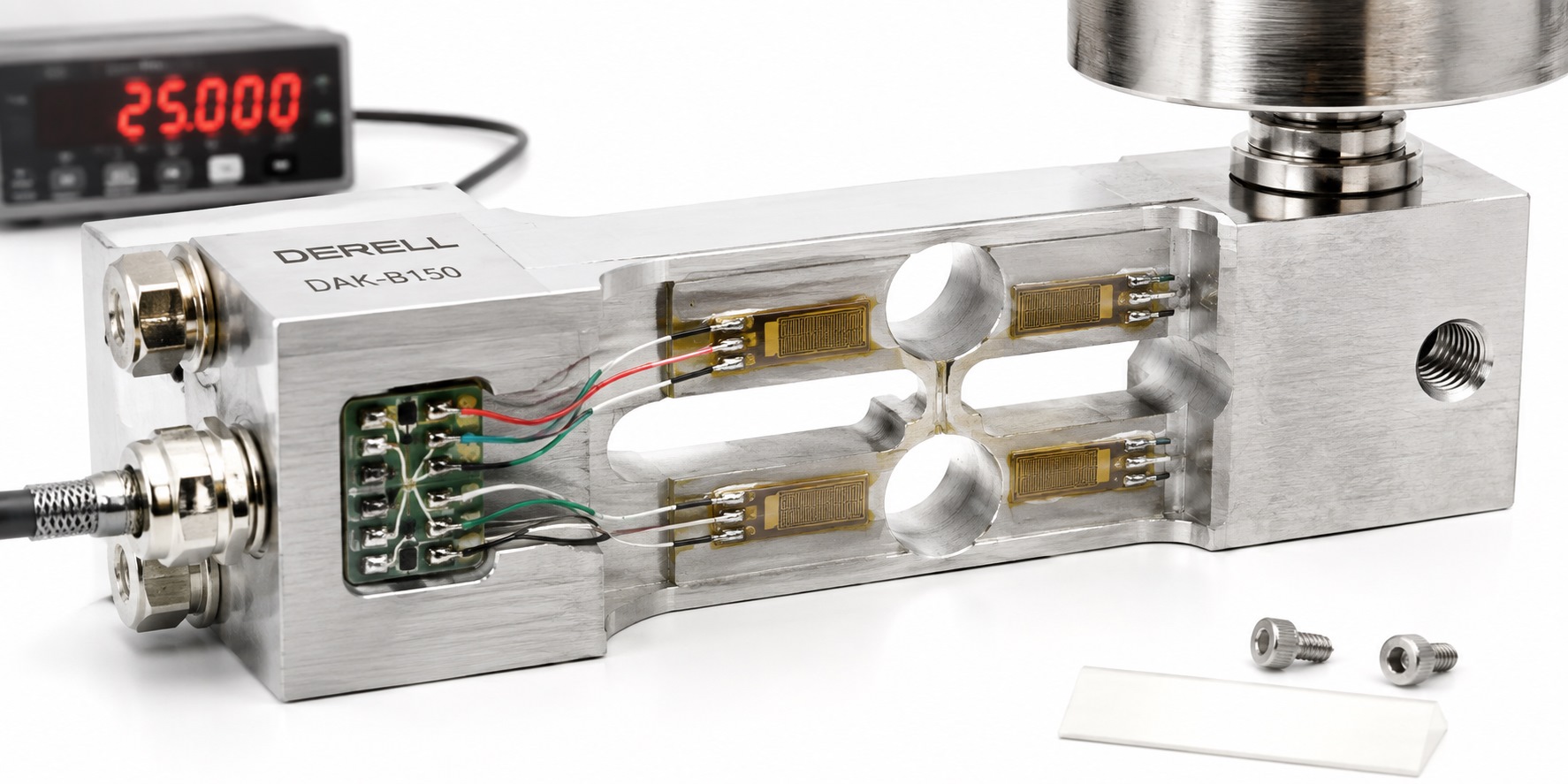
How does a load cell work? Trace the measurement from force to display

A load cell turns applied force into a measurable signal. In a common strain gauge design, the sensing body flexes slightly, bonded gauges change resistance, and an electrical bridge produces a small voltage. The instrument processes that voltage and applies calibration data to display a useful value. Our load cell overview explains the wider range of sensor designs.

Where the kilogram reading comes from

The bridge does not send a number labelled “kilograms”. The instrument establishes that relationship using zero and known reference loads. Suppose an unloaded system gives 0.15 mV and a 100 kg reference gives 10.15 mV. A 5.15 mV reading corresponds, with linear scaling, to 100 × (5.15 − 0.15) / (10.15 − 0.15) = 50 kg.

Subtracting the zero value matters: unloaded output need not be exactly zero. This two-point example explains scaling; a real calibration also checks intermediate loads, repeat readings and return to zero. Taring is not a substitute for calibration. The precision weighing guide and weight measurement guide consider the complete system. The sensor responds to force, so mass and weight remain distinct quantities.

Why the sensing body must flex

The metal body carries the applied load along its designed load path. Bonded strain gauges follow the small elastic deformation of that body. They are sensing elements, not structural supports. Gauge placement and body geometry determine how force produces strain; see the strain gauge load cell guide for the construction details.

Strain is a relative change in length: ε = ΔL / L. A 0.005 mm extension over 10 mm is 0.0005, or 500 µε. That is a length change of just 0.05%. Stress concerns force per unit area; strain describes deformation relative to an original dimension. The gauge measures strain.

The gauge’s electrical resistance changes with strain. Using ΔR / R = GF × ε, a 350 Ω gauge with GF = 2 changes by 0.35 Ω at 500 µε. The sign depends on whether that gauge experiences tension or compression. GF is the gauge factor; use the manufacturer’s actual value when calculating a real sensor response.

The bridge compares two voltages

A Wheatstone bridge has four resistive arms and two midpoint nodes. Excitation is applied across the top and bottom rails. The measured output is the difference between the two midpoint voltages. In this diagram, R1 is upper left, R2 lower left, R3 upper right and R4 lower right. Therefore VL = Vexc × R2 / (R1 + R2), VR = Vexc × R4 / (R3 + R4) and Vout = VL − VR.

With four equal 350 Ω arms and 5 V excitation, both midpoints are at 2.5 V and the ideal differential output is zero. At the animation’s 50 kg step, R1 and R4 are 349.65 Ω while R2 and R3 are 350.35 Ω. The midpoints become 2.5025 V and 2.4975 V: their difference is 5 mV.

This is an ideal full-bridge teaching model with matched tension and compression gauges, not a resistance specification for every load cell. Quarter- and half-bridge arrangements have different active elements and connections. Read the bridge formulas and bridge voltage calculation with their resistor labels in view.

Reading an mV/V specification

mV/V relates the rated output change to excitation voltage. For a 100 kg cell rated at 2 mV/V, 5 V excitation produces approximately 10 mV of change at rated load. In an ideal linear response, half that load gives a 5 mV change. The 2 mV/V rating does not state measurement accuracy. The permitted excitation range comes from the sensor’s technical documentation.

What the electronics add

A compatible instrument supplies excitation and reads the low-level analog signal. Amplification and filtering prepare it for measurement. In a digital instrument, an ADC converts it to numerical data, which calibration then scales into engineering units. A raw mV/V bridge requires a suitable bridge input. An ordinary 0–10 V analog input is not automatically suitable for direct connection.

A conditioner or weighing module may provide processed 4–20 mA, 0–10 V or supported digital data. The 0–10 V versus 4–20 mA guide and analog controller guide explain interface choices. Weighing controllers combine measurement with application functions; their capabilities depend on the model.

Excitation, signal and sense leads

EXC+/EXC− supply the bridge; SIG+/SIG− carry the differential signal. A six-wire cell adds SENSE+/SENSE−. With compatible instrumentation, these leads monitor excitation at the bridge and help compensate for losses in the excitation cable. A shield may be separate. Wire colours are not universal: match terminal functions using the sensor and instrument diagrams.

Why an apparently good signal can still give a wrong result

Mechanical contact, side forces, binding, vibration, temperature changes and electrical interference can disturb the result. A bridge arrangement may reduce some temperature effects; it does not cancel every error source. Stronger filtering can steady a display while slowing its response. Sensor selection and weighing data acquisition must account for the load direction and required measurement speed.

Do hydraulic and pneumatic cells use this circuit?

The explanation above concerns an electrical strain gauge bridge. Hydraulic cells relate force to fluid pressure; pneumatic cells use air pressure. How the result reaches an electrical system depends on the chosen transducer. The load cell types guide compares these different measurement technologies.

Two practical checks

Would more excitation improve the reading? Output can rise with excitation, but exceeding the specified limit is not a valid improvement. Heating and associated errors matter. Use the manufacturer’s recommended supply conditions.

Can a multimeter prove the sensor is healthy? It can assist with excitation and output checks. On a disconnected, unpowered bridge sensor, resistance measurements can be compared with specified values. Those checks do not establish full mechanical performance or calibration accuracy. The weighing FAQ covers further questions.

Continue with related guides

Technical references: FUTEK: load cell principles · NI: strain and bridge arrangements · OMEGA: strain gauges · OMEGA: measuring circuits · Interface: wiring and sense leads · FUTEK: signal conditioning · OMEGA: installation and calibration · TE Connectivity: load cell fundamentals