
What are the advanced interpolation algorithms for servo motors?
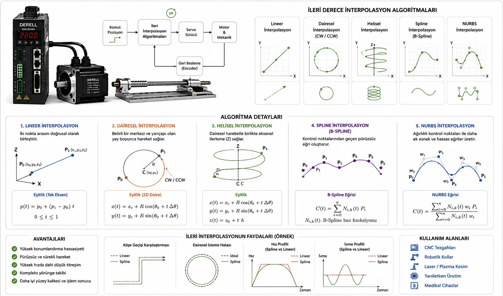
Planning smooth paths that a real machine can follow
Advanced interpolation generates the intermediate targets along a move. In a servo system, a CNC or motion controller usually performs that calculation; the servo drive and motor execute the resulting commands. Reaching the endpoint is only part of the job. Machining, dispensing and coordinated motion also require the right position and speed throughout the path.
1. Linear, circular and helical paths
Linear interpolation describes a straight move. Circular interpolation follows an arc, while helical interpolation combines circular motion with progress along a third axis, as in a spiral groove. In CNC machining, the interpolator generates coordinated targets from a shared path parameter. Axis control must preserve that relationship: starting all axes together does not guarantee the intended contour.
2. Cubic and quintic polynomial interpolation
Cubic polynomials can match endpoint positions and velocities under suitable boundary conditions. Quintic polynomials can also match endpoint accelerations. Hermite formulations use endpoint values and derivatives; Bézier formulations shape a curve through control points. Polynomial interpolation is also used in electronic cam tables. For coordinated axes, the connection conditions matter as much as the polynomial degree. A higher degree alone does not guarantee a better move.
3. Akima, cubic splines and B-splines
Splines build a path from connected curve segments. Akima splines pass through the specified points. Cubic splines can maintain first- and second-derivative continuity when constructed appropriately. B-splines use control points to shape the curve and generally do not pass through every control point. Passing through a waypoint and approximating a contour within tolerance are different requirements. Choose smoothing limits from the application's accuracy requirements.
4. NURBS and real-time parameter updates
NURBS interpolation describes a curve using its degree, control points, weights and knot vector. Suitable definitions can represent geometry such as circles exactly. However, equal parameter increments do not generally produce equal travel distances. Taylor-based and predictor–corrector interpolators calculate the next parameter value to achieve the required advance per cycle. Some implementations use Newton–Raphson corrections. These are numerical methods in the controller, rather than additional operating modes built into the motor.
5. Look-ahead and corner blending
Look-ahead examines upcoming path segments so the machine can adjust its speed before a demanding turn. Corner blending may insert an arc or spline between straight segments. A machine with finite acceleration cannot preserve an exact sharp corner while travelling through it at nonzero speed. Preserving the corner requires slowing down; rounding it requires an explicit contour deviation allowance. Planning limits should reflect the machine's dynamic behaviour.
Worked example: At 100 mm/s on a 50 mm radius arc, a 1 ms interpolation cycle gives approximately 0.1 mm of travel along the arc. If consecutive targets are joined by straight segments, the small-step chord error is approximately e ≈ (v × T)² / (8 × R), or 0.025 µm. At 5 ms it rises to about 0.625 µm. These are geometric sampling values; actual machine error can also include servo lag, structural deflection and backlash.
6. Jerk limits and adaptive feedrate scheduling
An S-curve profile determines how the move unfolds over time, rather than its geometric shape. Jerk is the rate of change of acceleration; limiting it can help reduce mechanical vibration. Jerk-limited and jerk-continuous motion are different properties. Adaptive feedrate scheduling adjusts speed to respect curvature and chord-error limits, pursuing dynamic performance within the machine's velocity, acceleration and jerk capabilities.
For circular motion, normal acceleration is a = v² / R. A speed of 200 mm/s on a 5 mm radius requires 8,000 mm/s². With an allowable normal acceleration of 2,000 mm/s², this constraint alone limits speed to 100 mm/s. Individual axis constraints may require a lower value.
7. Coordinating tool paths with robot joints
In robot motion planning, inverse kinematics converts the tool path into joint commands. A smooth tool motion can still demand high joint speeds. Time parameterization with joint limits addresses that problem. Methods such as TOTG assign timing under velocity and acceleration constraints; algorithms such as Ruckig can enforce jerk limits. When smoothing changes the path, collision clearance and contour compliance need to be checked again.
8. Making the calculated trajectory work on hardware
Real-time execution keeps target generation on schedule. An EtherCAT motion network can support synchronized axis operation, with timing configured for the application. Encoders and other feedback devices measure actual motion. Suitable loop tuning and feedforward help reduce tracking error. Even a well-planned curve cannot compensate for an incorrect load and transmission calculation.