
Dynamic modeling of servo motors
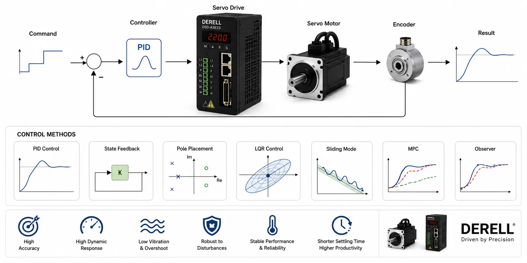
Predicting how a motor and its load respond
A dynamic model predicts how a servo motor's torque, speed and position change over time when voltage or current changes. Motor power alone cannot describe a servo system: the drive, transmission and load shape the response. A useful model supports motor selection and controller tuning, with predictions checked against measurements.
1. Mechanical dynamics: only net torque accelerates the load
J × dω/dt = Tm − TL − B × ω ; dθ/dt = ω
J is the total inertia referred to the motor shaft, Tm is motor torque, TL is external load torque and B is the viscous friction coefficient. θ denotes angular position and ω angular speed. Net torque produces acceleration; the motor must also overcome load and friction. Dry friction is not separately represented in this simple model. Use kg·m² for inertia, N·m for torque and rad/s for speed. Convert rpm using ω = 2π × n / 60.
2. The electrical model of a DC motor
u = R × i + L × di/dt + Ke × ω ; Tm = Kt × i
For a constant-field DC motor, u is terminal voltage, i is current, R is winding resistance and L is inductance. Ke and Kt are the back-EMF and torque constants. Inductance limits how quickly current changes, while back EMF increases the voltage required at speed. These relationships connect torque control with speed control. They should not be applied directly as the complete electrical model of a three-phase AC servo.
3. The d–q model for a three-phase servo
For a permanent-magnet synchronous motor, phase currents are transformed into id and iq components in a coordinate frame rotating with the rotor. Under a commonly used amplitude-invariant d–q convention, electromagnetic torque is:
Tm = (3/2) × p × [ψm × iq + (Ld − Lq) × id × iq]
p is the number of pole pairs, ψm is permanent-magnet flux linkage, and Ld and Lq are axis inductances. When Ld ≈ Lq, reluctance torque becomes small and torque is approximately proportional to iq. The detailed model also describes current dynamics and speed-dependent cross-coupling. Match the model to the datasheet's phase versus line, peak versus RMS and speed-unit conventions before comparing motor constants.
4. Refer every inertia to the same shaft
A load and transmission calculation needs a consistent mechanical reference. Define the reduction ratio as N = motor speed / load speed. For an ideal transmission, reflected load inertia = load inertia / N². Add gearbox and coupling inertias at the appropriate reference shaft. Electronic gearing changes command scaling; it does not physically reduce the load inertia.
Worked example: A 0.05 kg·m² load behind a 5:1 reduction reflects 0.002 kg·m² to the motor. With a motor inertia of 0.001 kg·m² and other rotating parts neglected, total J = 0.003 kg·m². Acceleration at 100 rad/s² requires 0.3 N·m. If the combined resisting torque at the motor shaft is 0.2 N·m at that instant, required motor torque is 0.5 N·m. With Kt = 0.5 N·m/A under a consistent current convention, approximately 1 A is required. This illustrates instantaneous demand; component selection must also consider peak and continuous operating limits.
5. Flexible mechanics need more than one inertia
A long shaft, belt or flexible coupling can make a single rigid-body model inadequate. A two-inertia model separates motor and load and represents their connection through stiffness and damping. It helps explain vibration and resonance. The motor encoder may report a steady position while the load oscillates. Load-side sensing, such as a linear encoder, provides a different view of the motion.
6. Transfer functions and state-space models
For the constant-parameter DC model with rigid mechanics, zero initial conditions, viscous friction only and TL = 0, the voltage-to-position transfer function is:
Θ(s) / U(s) = Kt / {s × [(L × s + R) × (J × s + B) + Ke × Kt]}
s is the Laplace variable; Θ(s) and U(s) are transformed position and voltage. A state-space representation can describe the same model using current, speed and position as states. For control-loop design, including the drive's inner current loop changes the effective plant. The motor transfer function and the complete closed-loop speed, torque and position response describe different systems.
7. Identify parameters, then test the predictions
Datasheet values provide a starting point. System identification uses measured behaviour to represent the actual machine. Steady-speed torque helps characterize friction; acceleration and deceleration records help identify inertia. Analyze current alongside feedback measurements. Auto-tuning can estimate some parameters, but should not be assumed to identify every mechanical effect. Validate the model with separate measurements that were not used to fit it, including different loads.
8. Include the drive and its operating limits
A practical model includes drive configuration, current and voltage limits, sampling and computational delays. Real-time cycle execution and communication timing influence when commands take effect. Add dry friction, backlash, temperature-dependent resistance and thermal limits when relevant. Deceleration modelling can also support assessment of regenerative energy flow. Additional detail is worthwhile when it improves predictions of the behaviour that matters.