
What is Electronic gearing?
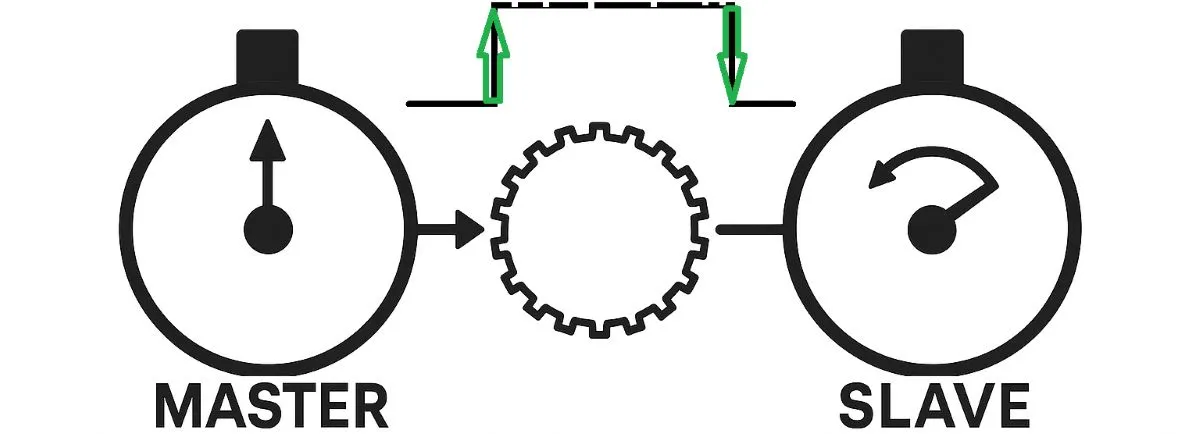
Make one axis follow another by a defined ratio
Electronic gearing establishes a defined ratio between a reference motion and the command for a follower axis. For example, one revolution of the reference can command two revolutions of the follower. The servo motor follows through its own servo drive and feedback loop. The reference can come from another motor, an external encoder, or a virtual axis generated by the controller.
Leader/follower and master/slave describe which axis provides the reference. A physical reference motor is optional: a PLC or motion controller can distribute a virtual reference to several axes. Depending on the servo system architecture, gearing may be implemented in the controller, in the drive, or across both.
Define the ratio before entering parameters
Let G = follower motion / reference motion = numerator / denominator. With matching position units and scales, the ideal relationship is ΔqF = G × ΔqR. Including the initial positions gives qF = qF0 + G × (qR − qR0). The reference and follower do not need to share the same zero position.
With G = 2, a 100° reference move commands 200° at the follower; with G = 1/2, it commands 50°. At a fixed ratio, the velocity relationship uses the same factor: a 60 rpm reference corresponds to 120 rpm or 30 rpm respectively. A negative ratio reverses the defined axis direction where supported. The denominator cannot be zero. A bare “1:2” is ambiguous unless the order of the axes is stated.
The displayed speeds are for illustration. During one reference revolution, the fast follower completes two revolutions and the slow follower completes half a revolution. Start restarts all axes from zero; stop freezes their current angles. This shows an ideal command relationship, without modelling motor inertia, following error or communication delay.
PPR, counts per revolution and internal units are different
If an incremental encoder’s 1,000 PPR specification means cycles per channel, a receiver using all four edges of the A/B signals obtains 4,000 counts per revolution. Single-edge, double-edge and quadrature decoding give different results. Manufacturers do not always use PPR, CPR, pulses and counts consistently, so establish the number of counts actually seen by the receiving input.
For a generic pulse scaling arrangement defined as internal position increments = input counts × B/A, the input counts required per motor revolution are C = E × A/B, where E is the drive’s internal increment count per motor revolution. E does not necessarily equal the encoder’s labelled PPR. Parameter direction and permitted ratios depend on the product; copying drive settings from another model can give the wrong scale.
A practical leadscrew calculation
Consider a directly coupled leadscrew with a lead of 5 mm per revolution. Suppose the electronic gear is configured for 10,000 command pulses per motor revolution. One pulse then commands 5 / 10,000 = 0.0005 mm, and a 20 mm move requires 20 × 10,000 / 5 = 40,000 pulses. That 0.5 µm value is the command increment; it does not establish the machine’s positioning accuracy.
At 300 rpm, f = n × C / 60 gives 50,000 pulses/s, or 50 kHz. Both the controller output and drive input must support that rate. Increasing pulses per revolution increases the required frequency at a given speed. For position commands sent over a network such as EtherCAT, the relevant constraints include command cycle time, scaling and timing performance; the pulse frequency calculation does not apply directly.
With a gearbox defined by i = motor speed / load speed, use P = travel × C × i / screw lead. At i = 2, the same 20 mm move requires 80,000 pulses. Applying the same gearbox conversion in both the PLC axis scaling and the drive scaling counts it twice and produces an incorrect travel distance.
Why can the physical axis lag behind a correct command?
Following error is the difference between commanded and measured position. Available torque, load inertia, mechanical compliance, backlash, tuning and signal quality affect positioning accuracy. Physical shafts can show transient error even when the command ratio is exact. Assessing dynamic performance requires acceleration, deceleration and load changes as well as steady-speed revolution counts.
For a fixed G, follower velocity and acceleration demands are the corresponding reference values multiplied by G. Increasing the ratio can therefore demand higher speed and acceleration. Zero physical error or unlimited synchronization cannot be assumed. Reaching a velocity ratio and arriving at a specified absolute position or phase are separate tasks; applications requiring phase alignment need a suitable synchronization method.
Check how gearing engages and disengages
The name MC_GearIn does not guarantee identical engagement behaviour across platforms. Beckhoff’s Tc2_MC2 MC_GearIn, for example, couples axes at standstill and provides other blocks for a moving reference. CODESYS SM3_Basic MC_GearIn can ramp the follower to the requested velocity ratio, without compensating the distance lost during engagement. After coupling, the control mode affects whether the relationship uses position or velocity values.
InGear indicates that the block’s defined coupling condition has been met; it does not independently prove that the workpiece is correctly phased. Likewise, MC_GearOut does not universally mean “stop the motor”: an axis may continue at its existing speed. Define the subsequent motion and stop separately. Arbitrarily changing the ratio or resetting the reference position while geared can also create an abrupt command change.
Commissioning and fault diagnosis
Establish the mechanical scale first: record screw lead, gearbox ratio, direction and actual travel per motor revolution. Check motor sizing and available torque against the required maximum speed and acceleration. Then confirm command format, electrical signal levels, receiver decoding and the maximum supported pulse frequency.
Measure at low speed: send a known pulse count and compare the drive’s received count, motor movement and actual load travel. A repeatable proportional distance error points first to scaling. Correct movement at low speed but errors at higher speed call for checks of frequency limits, wiring, signal noise and following error under load.
Test dynamic conditions: observe the position relationship through acceleration, deceleration, reversal, loss of reference and re-engagement. Modes that compensate buffered pulses can produce unexpected catch-up movement. Monitoring commanded position, actual position and error together helps separate the possible causes.
Where it fits, and where its limits begin
Printing, packaging, labelling and roll feeding are common industrial applications for motion derived from a shared reference. In multi-axis synchronization, electronic gearing suits a fixed ratio. If an axis must dwell, follow a special position curve, or change ratio during different parts of a cycle, use electronic camming or an appropriate motion profile and interpolation method. A changing winding diameter also means that a fixed rotational ratio alone cannot maintain constant surface speed or web tension.
Electronic gearing does not transmit mechanical power. It does not pass torque between axes or multiply torque through its electronic ratio; each motor drives its own load. It may reduce some mechanical linkages, but bearings, couplings, belts and screws still require maintenance. Overall energy efficiency depends on the motors, drives, mechanics and duty cycle. Enabling this function alone does not guarantee energy savings.
Related technical reading
Servo questions and answers; Servo drive configuration; Encoder and resolver feedback; Multi-axis motion coordination.