
How do I reduce a pump's energy consumption?
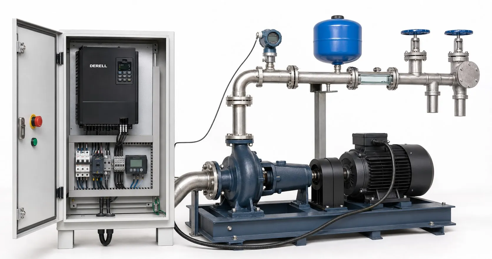
How to reduce pump energy use: measure, improve and verify
Lower pumping energy starts with defining the flow and pressure the process actually needs. Then check excess head, unnecessary operating time, pipe losses and control strategy. A drive or a high-efficiency motor alone cannot make the entire installation efficient. Confirm savings by measuring the electricity used to deliver the required service.
Measure energy at the supply
kW describes power; kWh describes energy. At constant power, energy = power × time. A system drawing 3 kW from the supply for ten hours uses 30 kWh. The kW rating on an electric motor usually specifies rated mechanical output, rather than the electricity recorded by the meter.
Use appropriate energy measurement equipment to log active input power and kWh. Include drive losses where a drive is fitted. A lower current reading alone does not prove lower energy consumption. Record flow, pressure, running time and demand as well. Electrical measurements require suitable instruments and qualified personnel.
What creates the power requirement?
Hydraulic power is the useful power transferred to the liquid. For water, an approximate calculation is Phydraulic (kW) = 0.002725 × Q × H, with Q in m³/h and H in metres. Total head includes the level difference, pressure requirement and flow losses; it is not simply the height of the pipe.
At 20 m³/h and 30 m total head, hydraulic power is about 1.64 kW. If the overall supply-to-liquid efficiency is assumed to be 60%, input power is approximately 1.64 / 0.60 = 2.73 kW. The efficiency is an example assumption, not a typical value for every installation. For a detailed pump power calculation, use the liquid density and actual efficiencies.
Work through the system in a practical order
1. Remove unnecessary flow and pressure. Check the required setpoint, the accuracy of the pressure sensor and its location. Persistent excess capacity calls for a review of pump selection. In suitable designs, an alternative impeller diameter may be considered using the manufacturer’s curves and permitted limits.
2. Reduce avoidable piping losses. Appropriate pipe diameter, fewer unnecessary bends and low-loss accessories can help. Check restricted strainers and filters; suitable differential pressure measurement can support monitoring. Lowering resistance in a fixed-speed system may increase flow, so reassess the operating point and controls before claiming a saving.
3. Address leaks and unnecessary recirculation. Supplying unused branches or returning excess flow through an unnecessary bypass can waste energy. Do not disable a minimum-flow protection line without assessing the pump requirements. Review the pump components and process together.
4. Recover performance lost through wear. Inspect the impeller, internal clearances, alignment and lubrication. After maintenance, repeat flow, pressure and electrical measurements. Investigate fault symptoms, new noise and overheating rather than accepting them as normal.
When does variable speed offer a strong opportunity?
For changing demand, assess a compatible VFD, suitable pump control and a correctly tuned PID loop. In friction-dominated centrifugal pumping systems, matching speed to demand can substantially reduce power. Maintain required pressure, minimum flow, cooling and the approved speed range.
Understand the cube-law example: With the same impeller, corresponding operating points and approximately unchanged efficiency, the affinity relationships are Q ∝ n, H ∝ n² and Pshaft ∝ n³. At 80% speed, the theoretical shaft-power ratio is 0.8³ = 0.512, a reduction of about 49%. This is not a guaranteed electrical saving for every installation.
Consider pumping to an elevated tank: the elevation difference remains when speed falls. Significant static head can make a direct cube-law savings estimate misleading. With submersible pumps and their drives, also check motor cooling and minimum speed. These centrifugal-pump relationships should not be transferred unchanged to positive displacement pumps.
5. Stage multiple pumps to suit demand. If one pump can deliver the required duty, review the need to run every unit continuously. Use the combined pump curve, system curve and each unit’s permitted operating region. When assessing multipump controls, account for start frequency as well as energy.
6. Assess the pump and motor as a package. A more efficient assembly can supply the same hydraulic duty with less electricity. Replacing the motor alone does not remove excess pressure dissipated across a valve. Include liquid properties and the actual operating point in the comparison.
Calculate the saving, then check the delivered service
Illustrative example: Average supply power falls from 3.0 kW to 2.2 kW while the system continues to provide the required service under comparable conditions. At 4,000 hours per year in both cases, annual use falls from 12,000 kWh to 8,800 kWh. The difference is 3,200 kWh/year, or approximately 26.7%. For the energy-cost calculation, multiply the difference by the applicable energy rate and assess other tariff charges separately.
If running time or pumped volume changes, total kWh alone can mislead. At comparable head, specific consumption = kWh / pumped m³ can be useful. Include the effect of taking longer to deliver the same volume. Assess investment cost, maintenance and downtime together; settings that shorten pump life may erase the apparent benefit.
Related topics
Explore more pumping topics: Pump systems · Pump FAQ · Pump control products
Sources: DOE / Hydraulic Institute / Europump — variable speed and static head · KSB — affinity laws · KSB — hydraulic power · KSB — efficiency and measurement boundaries · DOE — pipe sizing and friction losses · DOE — parallel pump operation · DOE — impeller trimming · DOE — pumping system performance sourcebook · DOE — maintenance and performance monitoring · DOE — testing system efficiency