
How is high dynamic performance achieved in servo motors?
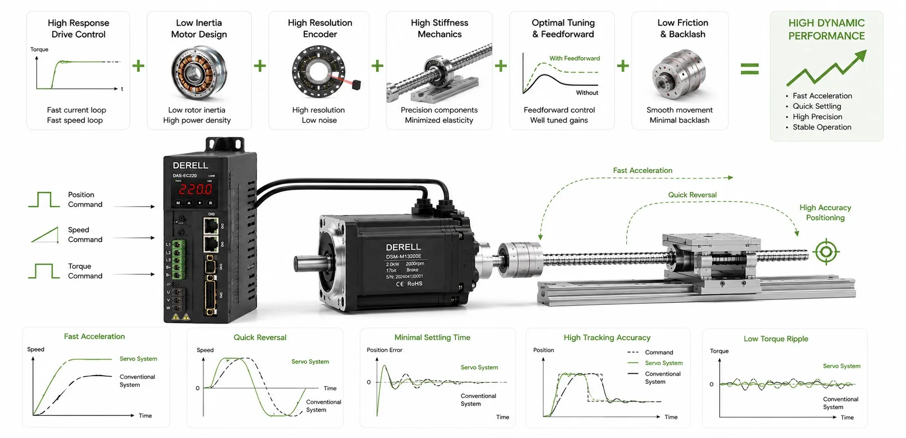
Fast moves that settle cleanly
High dynamic performance in a servo system means rapid acceleration, accurate command tracking, prompt recovery from load disturbances and short settling times. A servo motor's maximum speed says little about those capabilities on its own. The usable response comes from the motor, drive, mechanics, feedback and trajectory working together.
Define the response before choosing the settings
Following error is the difference between commanded and measured position during a move. Overshoot describes travel beyond the target. Post-move settling time is the additional time after the commanded trajectory ends for the axis to enter and remain inside a specified error band. State these limits alongside the required precision and accuracy. “Make it faster” is too vague to guide tuning or establish whether a change helped.
Acceleration starts with torque and inertia
For a simplified rotary system, α = Tnet / Jtotal. Net torque is the torque left to accelerate the system after resisting load and friction effects. Total inertia includes the motor rotor and the load referred to the motor shaft. A load and transmission calculation must account for mass distribution and transmission ratio, not just the weight of the moving part.
With a total inertia of 0.02 kg·m² and a constant net torque of 2 N·m, acceleration is 100 rad/s². Under those ideal conditions, reaching 300 rpm from rest takes approximately 0.314 seconds. Actual torque-speed limits, drive current limits and the motion profile change the result. Motor and drive sizing must therefore cover the required torque throughout the operating speed range.
Check repeatable duty, not only peak capability
A servo drive may supply enough current for one acceleration while repeated cycles overheat the motor. Assess peak torque, its permitted duration and the RMS torque or current over the complete duty cycle. Continuous capability also depends on speed, cooling, ambient temperature and mounting. A larger motor is not automatically a faster solution: its additional rotor inertia can increase the acceleration demand.
Deceleration returns mechanical energy to the DC bus. Depending on the supported architecture, that energy may require a correctly sized braking resistor, a shared bus or a regenerative supply. Inadequate energy handling can raise bus voltage and prevent the intended deceleration. Energy efficiency and rapid cycling need to be considered in the same design.
Mechanics determine how far tuning can go
Loose couplings, compliant belts, gearbox backlash and weak structures can produce mechanical vibration. Removing unnecessary moving mass, improving stiffness and correcting alignment may achieve more than increasing gains. There is no universal acceptable motor-to-load inertia ratio for every machine; compliance and the required response matter too. Dynamic modeling helps identify the load behavior and dominant resonances that constrain performance.
Balance feedback gains, feedforward and filters
Auto-tuning can establish initial settings, but verify them with representative moves. During drive configuration, account for the interaction of current, velocity and position loops. Higher control bandwidth can improve response, while excessive controller gain can amplify noise or excite resonances. A bandwidth figure in a catalog does not describe the response of the complete loaded machine.
Velocity and acceleration feedforward use the planned trajectory to reduce the error that feedback must correct. Their coefficients must suit the actual load and speed and torque control structure. A notch filter can attenuate a measured resonance, provided its frequency, width and depth are appropriate. A low-pass filter can reduce noise while adding delay. Assess both vibration and response after changing signal filtering.
Optimize the move and the settling period together
In speed, torque and position control, the rate of acceleration change matters as well as acceleration itself. This rate is called jerk. An S-curve profile smooths acceleration transitions and can reduce mechanical excitation, but may lengthen travel time depending on the chosen limits. Evaluate interpolation and trajectory settings against the complete cycle.
Consider an illustrative comparison: one setting needs 350 ms for travel and 120 ms to settle, totaling 470 ms. Another needs 380 ms for travel and 40 ms to settle, reaching a usable position in 420 ms. Arriving at the target first does not necessarily produce the shortest production cycle.
Measure the right position at the right time
Feedback quality involves accuracy and latency as well as encoder resolution. Motor-shaft position may differ from load position across a compliant transmission. In suitable applications, a linear encoder on the load can measure load position directly, although a dual-feedback control structure needs its own tuning. Consistent real-time execution and EtherCAT timing also matter. Verify multi-axis motion by inspecting the complete path.
Prove the result under the actual workload
Record following error, settling time, overshoot, peak and RMS current, and temperature at minimum and maximum load. Include stops, reversals and repeated cycles. Adaptive control may help when load dynamics change, but cannot supply missing torque or repair faulty mechanics. Keep results for comparison with later maintenance records, so deterioration can be detected rather than hidden by further tuning.