
What are the applicability and advantages of adaptive control algorithms in servo systems?
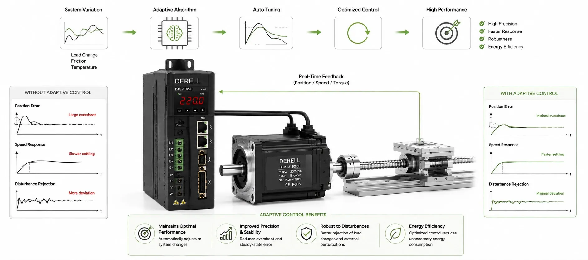
Keeping servo response consistent as the load changes
A servo system tuned for one operating condition may respond differently when payload, friction or mechanical dynamics change. Adaptive control updates controller parameters or a plant model using information collected during operation. The goal is to maintain the required motion response across those changes. Its value depends on a suitable design and measured performance on the machine.
What information does the controller use?
An adaptive function in the servo drive or motion controller may use commands, current-derived torque estimates and feedback. Position and velocity obtained from an encoder are compared with the expected response. Depending on the dynamic model, the algorithm may adjust feedback gains, feedforward coefficients, or estimated inertia and friction. The update rule must distinguish useful evidence from measurement noise.
A load change expressed in torque
Suppose the equivalent inertia referred to the motor shaft is 0.01 kg·m². At an angular acceleration of 100 rad/s², the acceleration torque is 1 N·m, from T = J × α. Increasing the inertia to 0.02 kg·m² raises that component to 2 N·m for the same acceleration. Friction and gravity are excluded here; a complete load and transmission calculation must account for them separately.
An updated inertia estimate can improve acceleration feedforward in torque control, leaving less error for the feedback loop to correct. It does not follow that every gain should double when inertia doubles. Mechanical compliance, delay and controller structure also shape speed and torque response. This is why adaptation needs a defined control law rather than an unrestricted gain adjustment.
How does it differ from automatic tuning?
Auto-tuning may run a commissioning test and produce settings that remain fixed afterward. Other functions update settings while the machine operates. Check the product documentation to establish which behavior is provided. Gain scheduling selects or interpolates predefined settings using variables such as speed or load; by itself, it does not learn unknown parameters online. During drive configuration, identify what an “automatic” function actually changes.
Which approaches are available?
A self-tuning controller estimates plant parameters and uses them to calculate control settings. Recursive least squares (RLS) is one option for online estimation when the model and data are suitable. An inertia estimate, for example, can support calculations for PID gains or feedforward. RLS supplies estimates; a separate control design determines how to use them.
Model reference adaptive control (MRAC) aims to make the actual system follow a chosen reference-model response. Direct MRAC updates controller gains; indirect MRAC first estimates plant parameters. Adaptive model predictive control (MPC) updates its prediction model and can incorporate specified constraints when calculating commands. These are design approaches, not features that can be assumed to exist in every commercial servo drive.
Where is adaptation worth considering?
Potential candidates include robot axes carrying different payloads, mechanisms with interchangeable tooling and winding systems whose roll diameter changes. The relevant question is whether the changing dynamics materially affect performance. A constant-load axis may already meet its target with fixed gains. For machines using interpolation and multi-axis coordination, evaluate the complete path while individual axis settings change.
What benefits can be demonstrated?
A successful implementation may deliver smaller tracking errors, more consistent settling times, less overshoot and fewer manual adjustments after load changes. These improvements can support precision and accuracy and dynamic performance. Reduced unnecessary oscillation may also contribute to energy efficiency, but adaptive control does not imply a universal energy-saving percentage.
What limits its practical use?
Reliable measurements and informative motion data are essential. A single steady-speed measurement may not distinguish inertia from friction. Some estimators require sufficient excitation to identify parameters. Convergence to the true parameter values and a small tracking error are different outcomes. Signal noise and filtering delay can affect the quality of the estimates.
The design must address adaptation rate, parameter bounds and closed-loop stability. Aggressive updates can follow noise; slow updates can lag behind a changing load. Torque saturation can distort the information used by an estimator. Computation must meet the real-time control deadline. Adaptation should not be expected to repair backlash, damaged components or every source of mechanical vibration.
How should the machine be tested?
Compare identical moves at minimum and maximum load, with adaptation disabled and enabled. Record tracking error, settling time, overshoot, peak and RMS current, and the estimated parameters. Include the first move and the transition after a load change, rather than judging only the final steady response. Preserve these results in maintenance records. Correct motor and drive sizing remains essential: adaptation cannot increase the motor's torque or thermal limits.