
What is the device's response time?
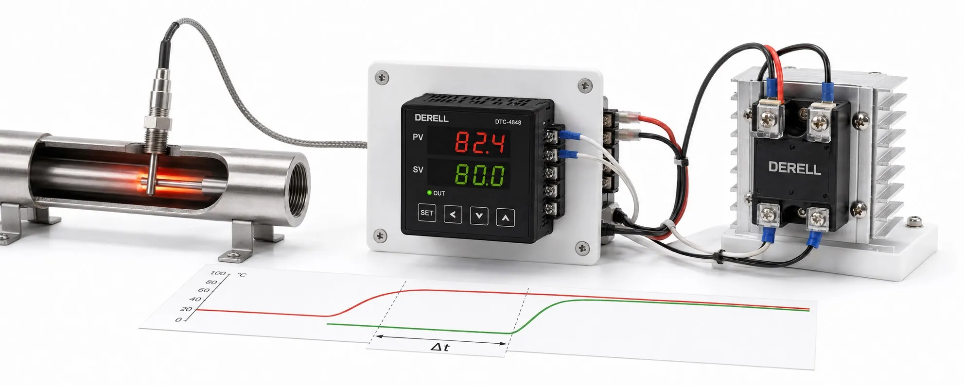
Fast controller decisions do not make a process heat instantly
A temperature controller has no single universal response time. Reading an input, sensing a temperature change, changing the control output and bringing the product to its target are different time measures. Fast electronics do not make a large tank or furnace change temperature equally quickly. First establish which time measure you are comparing.
Time measures that are often confused
| Time measure | What does it describe? |
|---|---|
| Sampling / calculation interval | Time between input acquisition or control-computation updates. |
| Sensor response | How the probe follows an actual temperature change, defined using a threshold such as t63 or t90. |
| Output cycle | The switching period for time-proportioning control; distinct from the sampling interval. |
| Dead time L | Delay before the measured response starts changing after an applied change. |
| Rise time | Usually the time to move from 10% to 90% of the total change. |
| Settling time | Time until the response enters the specified tolerance band and remains within it. |
Check the datasheet for the input type, filter setting and response threshold associated with a quoted time. For example, Yokogawa's TC10 FAQ specifies an I/O response of approximately 2 seconds or less at 63% response under its stated electrical-input change. This does not mean a furnace reaches its setpoint in two seconds. Assess temperature-measurement delay separately from the process's thermal response.
Why do the sensor and mounting matter?
Alongside sensor compatibility, consider probe diameter, sheath, thermowell, immersion depth and flow conditions. A thin thermocouple directly exposed to the process can respond quickly, but a heavily sheathed thermocouple is not necessarily faster than a small RTD. The thermocouple or RTD label alone does not determine response time. Gaps and poor thermal contact in the installation can delay the measurement.
Measurement accuracy and speed are different properties. An input filter can suppress fluctuations while adding delay. If the sensor measures near the heater rather than the actual product, a fast display change does not establish equally fast heating of the product.
An example using time constant and dead time
To illustrate system dynamics, consider a first-order model with dead time approaching 100 °C from 20 °C after a power step. Let the dead time be L = 5 s and the time constant τ = 30 s. For t < L, temperature remains at 20 °C; for t ≥ L, use T(t) = 20 + 80 × [1 − e−(t−5)/30].
At 35 seconds, approximately 63.2% of the total 80 °C change is complete, giving about 70.6 °C. The response reaches approximately 95% at 95 seconds and 99% at 143 seconds. The 10–90% rise time is τ × ln(9) ≈ 65.9 s; a pure dead time cancels from the difference between these threshold times. These are results for the example model, not guaranteed controller specifications.
For an ideal monotonic first-order response, 3τ gives approximately 95.0% and 5τ approximately 99.3% after the dead time. Do not apply this rule to every control algorithm or oscillating closed-loop system. State whether the settling band is a percentage of the total change or a fixed temperature tolerance. First entering the band is insufficient; the response must remain inside it.
PID tuning and the output cycle
In PID temperature control, assess the P, I and D effects together. Pushing gains solely for a fast rise can increase overshoot or oscillation. The goal is stable operation within the product's permitted time and tolerance. If heater power, thermal capacity, losses or heat transfer limit the response, PID tuning alone cannot remove that physical constraint.
For time-proportioning control, the output cycle differs from the measurement interval. With a 10-second cycle and 30% output, a simple implementation gives approximately 3 seconds on and 7 seconds off. Unnecessarily shortening a mechanical relay or contactor cycle increases switching operations; a suitable SSR may support more frequent switching. Select the cycle according to the output device and process instructions.
Editor's note: “100 ms sampling” does not mean “temperature corrected in 100 ms”. It may describe input or calculation updates. Sensor lag, filtering, the output device and thermal inertia still matter, and these effects do not all behave as fixed delays that can simply be added together.
How can you measure and improve the response on site?
From a defined starting condition, apply a small, controlled setpoint change and log the setpoint, measured temperature and output percentage with timestamps. Keep the load, environment, filter and output cycle consistent. Report rise time, overshoot and settling time within the stated band together. When logging through communications, distinguish the polling interval from the instrument's actual sampling interval.
With PLC-based PID, also check task timing and data freshness. Identifying a process using a power step differs from a closed-loop setpoint test. For slow response or oscillation, first investigate sensor location, filtering and actual output power. During maintenance, check loose probe contact and heater performance. Evaluate energy efficiency across the heating or cooling process rather than from the controller's own consumption alone.